Plotting Events
Create event histograms and adjust color, display mode, bins, navigation, and plot output.
5. Plotting Events
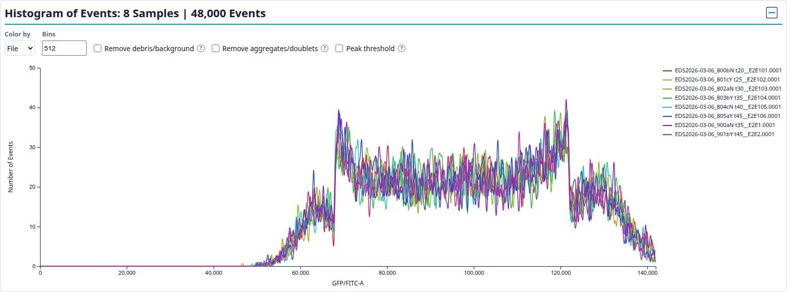
Click Plot Channel Events to load the selected channel's data for every checked row in the metadata table and draw an overlaid event histogram (x-axis: the chosen channel; y-axis: number of events). The plot panel title reports the number of plotted samples and total included channel events.
The plot stays live afterward: checking or unchecking a row in the metadata table immediately adds or removes its curve — unchecking a row does not discard its already-loaded data, so re-checking it is instant. After the first plot, the button turns blue as a reminder that a channel is already plotted; click it again any time to refresh.
Color by, display, and bins
- Color by — File gives every sample its own color; Strain groups samples sharing the same Strain annotation under one color.
- Display — choose smoothed curves, histogram bins, or both. This applies in both the Overlay and Ridge views.
- Bins — the histogram bin count, chosen on a slider with four stops (128, 256, 512, 1024; default 256). A larger bin count makes narrower bars and can reveal finer structure, but also makes curves noisier when event counts are low; a smaller count smooths the curves and makes broad trends easier to compare, but can hide small peaks or shoulders. The slider colours the chosen stop green/amber/red by how many events fall in each bin for your smallest sample, and marks the recommended stop with a teal outline.
- View — Overlay superimposes every plotted sample on one axis; Ridge stacks each sample as its own small histogram (with its fit) for side-by-side review.
Choosing a bin count
The bin count only makes sense relative to how many events you have — they aren't independent settings. The x-axis is a continuous range of values, and a bin is one equal-width slice of it; the histogram's height at that slice is simply how many events fell inside it. On average:
events per bin ≈ total events ÷ number of bins
More bins spreads the same events thinner, so each bin's count gets small and jittery — the curve looks noisy, and that noise can look like a real peak that isn't there. Fewer bins packs more events into each slice (smoother), but real structure that's close together — for example a small shoulder right next to the G1 peak — can blur into one blob.
| Events per bin | What it means |
|---|---|
| Fewer than 20 | Too sparse — random noise can look like a real peak. |
| 20–50 | Usable, but getting noisy. |
| More than 50 | Good balance of detail and stability. |
128 bins is always shown as a caution stop, even with plenty of events per bin, because it can be coarse enough that G1, S, and G2/M blur into each other.
For example, a sample with about 60,000 events breaks down like this:
| Bins | ~Events per bin | Rating |
|---|---|---|
| 128 | ~469 | Caution — coarse; peaks can merge |
| 256 | ~234 | Good |
| 512 | ~117 | Good |
| 1024 | ~59 | Good, but close to the edge |
The slider marks one stop with a teal outline: the finest (most detailed) bin count that still stays in the good range for whichever plotted sample has the fewest events, so no sample ends up under-supported. Fewer events overall means fewer bins are recommended; more events means you can afford finer detail.
Where these thresholds come from
These are a practical, conservative guideline, not a formally published statistical standard specific to flow cytometry histograms. The underlying idea — that sparse bins introduce counting noise — is well established (a classical rule of thumb for count-based histograms calls for at least around 5 events per bin for the statistics to behave); PhaseFinder's floor of 20 is intentionally well above that minimum. Treat the colour coding as guidance, not proof, and use your own judgment about whether a fit looks right.
Above the plot, a toolbar (camera, pan, zoom in, zoom out, autoscale, home) lets you download the plot as an image (SVG, PDF, PNG, or JPEG), or download a printable HTML analysis report containing the plot and metadata/results table. Drag to pan, hold Shift and drag to zoom into a rectangle, use the mouse wheel to zoom, and double-click empty space to reset. Panning and zooming only change the view — they never re-run detection or a fit.
Event-quality masks and contamination terms are controlled by the pre-modeling QC filters below, so every correction has a visible control and diagnostic readout.